Methane (CH4) Partial Column - Scatter Plot

Create a scatter plot of Methane CH4 partial column retrieved from the Cross-track Infrared Sounder (CrIS JPSS-1) global observations.

import numpy as np
from netCDF4 import Dataset

import matplotlib.pyplot as plt

from mpl_toolkits.basemap import Basemap

# Open the netCDF file
dataset = Dataset('./data/TROPESS_CrIS-JPSS1_L2_Summary_CH4_20230516_MUSES_R1p20_FS_F0p6.nc', 'r')

# Read the data from your variables
latitude = dataset.variables['latitude'][:]
longitude = dataset.variables['longitude'][:]
x_col_p = dataset.variables['x_col_p'][:]

dataset.close()

# Specify figure size (in inches)
plt.figure(figsize=(12, 8))  

# Create a basemap instance
m = Basemap(projection='cyl', resolution='l', 
            llcrnrlat=-90, urcrnrlat=90,  # set latitude limits to -90 and 90
            llcrnrlon=-180, urcrnrlon=180)  # set longitude limits to -180 and 180

m.drawcoastlines(linewidth=0.2)
m.drawcountries(linewidth=0.2)

# Draw parallels (latitude lines) and meridians (longitude lines)
parallels = np.arange(-90., 91., 30.)
m.drawparallels(parallels, labels=[True,False,False,False], linewidth=0.3)

meridians = np.arange(-180., 181., 60.)
m.drawmeridians(meridians, labels=[False,False,False,True], linewidth=0.3)    

# Standard catter plot
# Transform lat and lon to map projection coordinates
x, y = m(longitude, latitude)

# Plot the data using scatter (you may want to choose a different colormap and normalization)
sc = m.scatter(x, y, c=x_col_p, cmap='jet', s=10)

# Add a colorbar
cbar = m.colorbar(sc, location='bottom', pad="10%")
cbar.set_label('x_col_p')

plt.show()

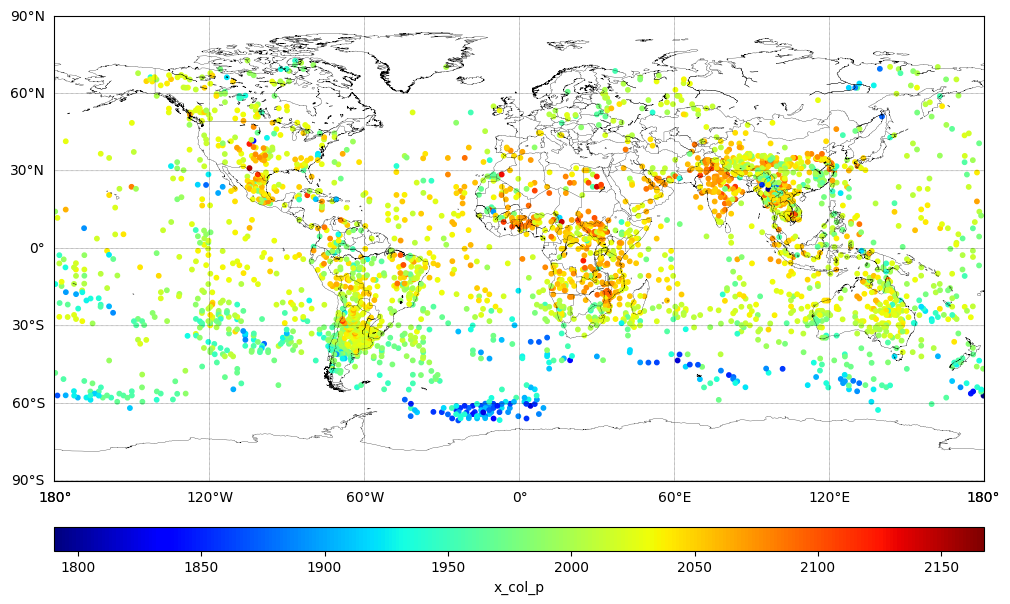
Bias corrected column-averaged dry air mixing ratio of Methane for the partial column (x_col_p) from 826 hPa to Top of Atmosphere (TOA) in ppbv - May 16th, 2023.