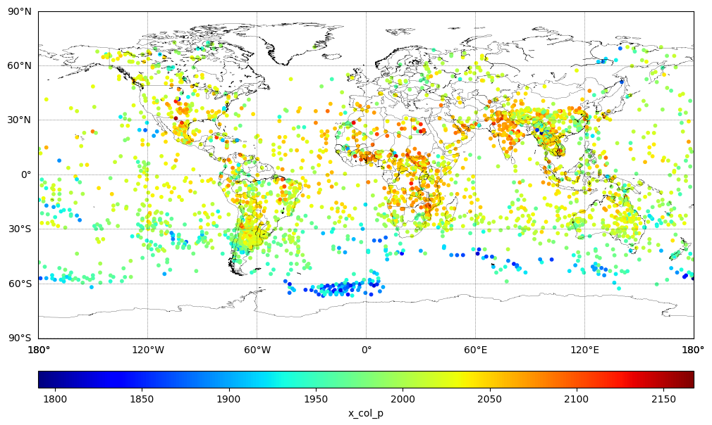
Methane Free Tropospheric Column (XCH4)

Plot the partial column variable x_col_p a.k.a. XCH4, in ppbv. The partial XCH4 has been pre-calculated for the pressure levels between 826 hPa and the Top of Atmosphere (0.1 hPa). This value is also known as the free tropospheric column mixing ratio.

For Methane concentration retrieved from CrIS JPSS-1 global observations.

Import packages

import numpy as np
from netCDF4 import Dataset

import matplotlib.pyplot as plt

from mpl_toolkits.basemap import Basemap

Read data variables

# Open the netCDF file
dataset = Dataset('./data/TROPESS_CrIS-JPSS1_L2_Summary_CH4_20230516_MUSES_R1p20_FS_F0p6.nc', 'r')

# Read the data from your variables
latitude = dataset.variables['latitude'][:]
longitude = dataset.variables['longitude'][:]
x_col_p = dataset.variables['x_col_p'][:]

dataset.close()

Create plots

# Specify figure size (in inches)
plt.figure(figsize=(12, 8))  

# Create a basemap instance
m = Basemap(projection='cyl', resolution='l', 
            llcrnrlat=-90, urcrnrlat=90,  # set latitude limits to -90 and 90
            llcrnrlon=-180, urcrnrlon=180)  # set longitude limits to -180 and 180

m.drawcoastlines(linewidth=0.2)
m.drawcountries(linewidth=0.2)

# Draw parallels (latitude lines) and meridians (longitude lines)
parallels = np.arange(-90., 91., 30.)
m.drawparallels(parallels, labels=[True,False,False,False], linewidth=0.3)

meridians = np.arange(-180., 181., 60.)
m.drawmeridians(meridians, labels=[False,False,False,True], linewidth=0.3)    

# Standard catter plot
# Transform lat and lon to map projection coordinates
x, y = m(longitude, latitude)

# Plot the data using scatter (you may want to choose a different colormap and normalization)
sc = m.scatter(x, y, c=x_col_p, cmap='jet', s=10)

# Add a colorbar
cbar = m.colorbar(sc, location='bottom', pad="10%")
cbar.set_label('x_col_p')

plt.show()