Brazilian Fires - Carbon Monoxide (CO) - CrIS JPSS-1

Total Column - gridded data (14km x 14km) plots

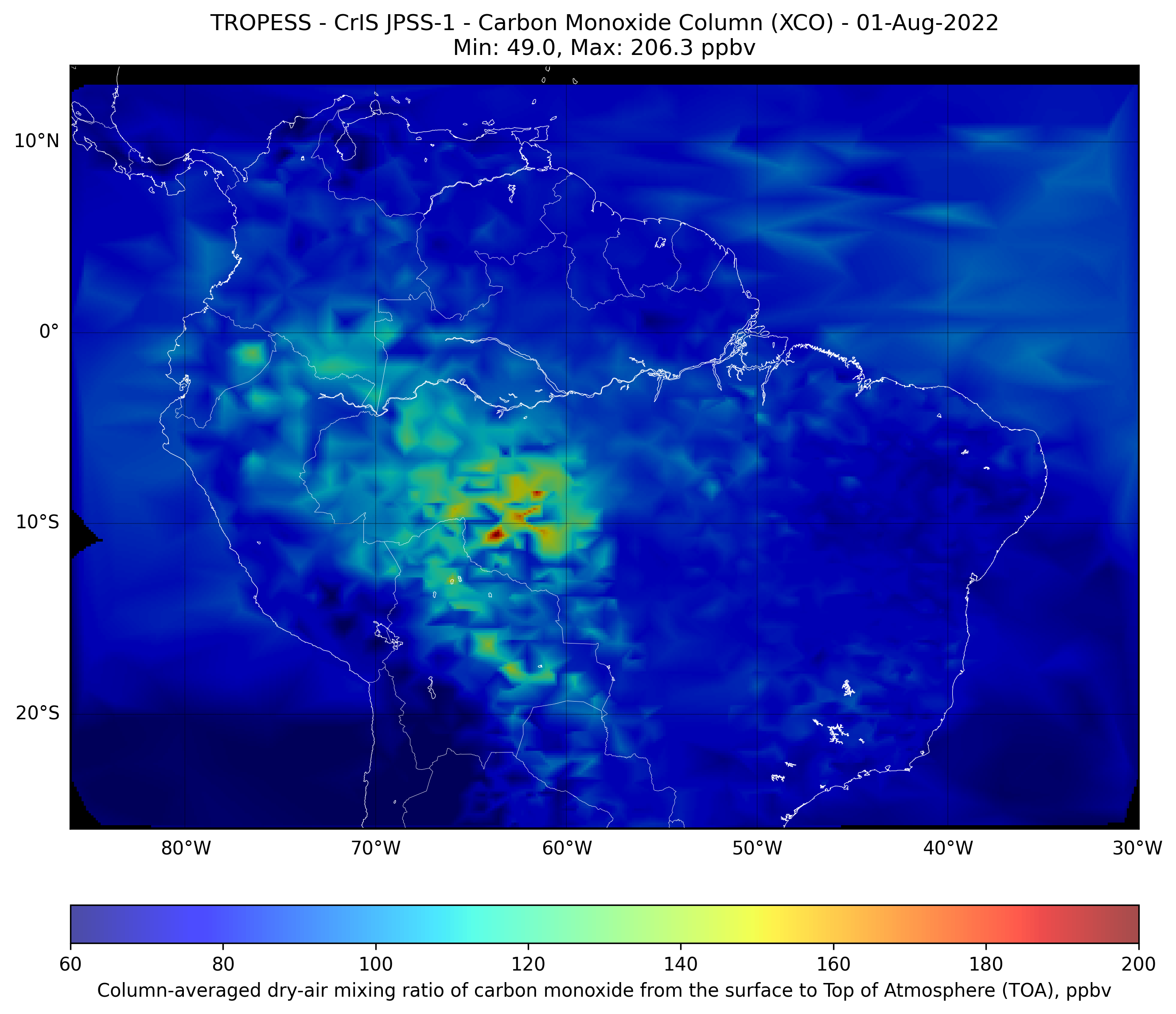
This code plots the Carbon Monoxide (CO) total column for each day from 01-Aug-2022 to 31-Aug-2022.

import datetime
import contextlib
from pathlib import Path

import pandas as pd

import numpy as np
from netCDF4 import Dataset

import matplotlib.pyplot as plt

from mpl_toolkits.basemap import Basemap

from scipy.interpolate import griddata
from scipy.spatial import cKDTree

import imageio.v2 as imageio

# Specify date range
start_date = datetime.date(2022, 8, 1)
end_date = datetime.date(2022, 8, 31)

# Loop through the date range and plot Carbon Monoxide for each day
for current_date in pd.date_range(start_date, end_date):
    data_file_date = current_date.strftime("%Y%m%d")
    
    # We may not have data for certain days    
    data_file_path = Path(f'./data/TROPESS_CrIS-JPSS1_L2_Summary_CO_{data_file_date}_MUSES_R1p17_FS_F0p6.nc')
    if not data_file_path.exists():
        continue

    # Open the netCDF file
    dataset = Dataset(data_file_path.as_posix(), 'r')

    # Read the data from your variables
    latitude = dataset.variables['latitude'][:]
    longitude = dataset.variables['longitude'][:]
    x_col = dataset.variables['x_col'][:]

    dataset.close()

    # Filter the data for South America only
    latitude_max = 14.0
    latitude_min = -26.0
    longitude_max = -30.0
    longitude_min = -86.0

    south_america_only = np.where(
        (latitude > latitude_min) & (latitude < latitude_max) & 
        (longitude > longitude_min) &(longitude < longitude_max)
    )[0]

    latitude = latitude[south_america_only]
    longitude = longitude[south_america_only]
    x_col = x_col[south_america_only]

    # Calculate width and height
    aspect_ratio = (longitude_max - longitude_min) / (latitude_max - latitude_min)
    w = 3600; h = w / aspect_ratio

    # Specify figure size (in inches)
    dpi = 300; 
    plt.figure(figsize=(w / dpi, h / dpi))  

    # Create a basemap instance
    m = Basemap(projection='cyl', resolution='i',
                llcrnrlat=latitude_min, urcrnrlat=latitude_max,  # set latitude limits to -56 and 24
                llcrnrlon=longitude_min, urcrnrlon=longitude_max)  # set longitude limits to -96 and -30

    m.drawmapboundary(fill_color='black')
    m.drawcoastlines(linewidth=0.3, color='white')
    m.drawcountries(linewidth=0.2, color='white')

    # Draw parallels (latitude lines) and meridians (longitude lines)
    parallels = np.arange(-90., 91., 10.)
    m.drawparallels(parallels, labels=[True,False,False,False], linewidth=0.3)

    meridians = np.arange(-180., 181., 10.)
    m.drawmeridians(meridians, labels=[False,False,False,True], linewidth=0.3)

    # Get CrIS pixel size in degrees, pixel is 14 x 14 km, 1 degree is roughly 111.1 km
    cris_pixel_size_deg = 14.0 / 111.1 

    # Get the grid for the interpolated values
    grid_lat, grid_lon = np.mgrid[-26:13:cris_pixel_size_deg, -86:-29:cris_pixel_size_deg]

    # Interpolate the data using griddata
    grid_x_col = griddata((latitude, longitude), x_col, (grid_lat, grid_lon), method='linear', rescale=True)

    # Find the distance to the nearest original point for each point in the interpolated grid
    tree = cKDTree(np.vstack((latitude, longitude)).T)
    dist, _ = tree.query(np.vstack((grid_lat.ravel(), grid_lon.ravel())).T)

    # Reshape the distance array to have the same shape as the x_col grid
    dist_grid = dist.reshape(grid_x_col.shape)

    # Mask the interpolated values that are too far from any original point
    max_distance_degrees = 3.0
    grid_x_col[dist_grid > max_distance_degrees] = np.nan

    # Plot the interpolated data using pcolormesh instead of scatter
    sc = m.pcolormesh(grid_lon, grid_lat, grid_x_col, latlon=True, cmap='jet', alpha=0.7, vmin=60.0, vmax=200.0)

    # Add a colorbar
    cbar = m.colorbar(sc, location='bottom', pad="10%")
    cbar.set_label('Column-averaged dry-air mixing ratio of carbon monoxide from the surface to Top of Atmosphere (TOA), ppbv')

    # set plot title
    title_date = current_date.strftime("%d-%b-%Y")
    title_min = np.min(x_col)
    title_max = np.max(x_col)
    plt.title(f'TROPESS - CrIS JPSS-1 - Carbon Monoxide Column (XCO) - {title_date}\nMin: {title_min:.01f}, Max: {title_max:.01f} ppbv')

    # Save figure to PNG file
    plt.savefig(f'./images/TROPESS_Brazilian-Fires_CrIS-JPSS-1_XCO_{title_date}.png', dpi=dpi, bbox_inches='tight')

    plt.close()

Now generate an animated GIF from the saved figures.

timelapse_start_date = start_date.strftime("%d-%b-%Y")
timelapse_end_date = end_date.strftime("%d-%b-%Y")
timelapse_file = f'./images/TROPESS_Brazilian-Fires_CrIS-JPSS-1_XCO_Timelapse_{timelapse_start_date}_{timelapse_end_date}.gif'

# Path to the directory where the images were saved in the previous step
img_dir = Path('./images')

# Get all file names in the directory
files = sorted([img for img in img_dir.glob("TROPESS_Brazilian-Fires_CrIS-JPSS-1_XCO_*.png")])

# Read the images and add to a list
with contextlib.redirect_stdout(None):
    images = []
    for filename in files:
        images.append(imageio.imread(filename))

    # Save the images as an animated gif
    # duration is the time spent on each image (in milliseconds)
    imageio.mimsave(timelapse_file, images, duration=1000.0, loop=0)  

First day

Timelapse